Note: I assume you already know some λ-calculus, at least how to apply an expression to a function. If you need a primer, look here, especially the section called “Function application”.

If you’re anything like me, you are 1) interested in λ-calculus, and 2) a bit dissatisfied. You may or may not know about the Y-combinator and its immense importance. It is a construct that enables recursion, and as a result, causes some problems. There are also other cool combinators. And here’s how they are usually explained to me:

Clever person: The Y-combinator looks like this. [Shows me some lambda expression.]

Me: Oh cool, how does it work?

CP: You just apply it to anything like this, and causes recursion!

Me: Huh. But why?

CP: Why it causes recursion? Just try it and you will see it works!

Me: Yeah, but… How? How did you come up with this?

CP: I didn’t. But it works!

Wholly unsatisfactory. I want to understand how I could construct it. I don’t think Haskell Curry just stared at the problem of recursion in λ-calculus until a really cool expression jumped up at him an introduced itself as “Mr. Y”. Or maybe it did – logicians, am I right? – but I’m an engineer, and I want ways, methods, and techniques.

An aside about math and proofs

As anyone who has ever tried to construct a proof knows, it’s not a straightforward process. It requires various degrees of knowledge, strategy, imagination, inspiration, and luck to come up with a good proof. Constructing a proof may take many turns and dead ends, but in the end, it usually comes down to making some sound decisions along the way and looking in just the right direction at just the right time. But that is not how proofs are presented in books. They work more like a map, which is great if you’re trying to just find your way, but worthless if you’re trying to learn the art of finding your own way in unknown territory (which is really the point of learning math at all).

The thing that often bugs me about most resources on λ-calculus¹ is that they tend to be “clever”. They show you a construction, and that it works. But more than in the other branches of math I’ve covered, the constructions seem to appear out of thin air. That makes it both more boring to learn, and harder to remember (the number of times I’ve looked up the Y-combinator just to forget it 3 seconds later…)

The Y-combinator

A combinator is just a lambda expression with no free variables. The point of having combinators is that you can combine them (duh) and in theory, work only with a set of ready-made combinator functions and never worry about the details of making your own λ-abstractions, etc. It becomes more like doing arithmetic: you are applying multiplication * without worrying too much of the definition, just by knowing how that specific function it is supposed to transform its inputs into an output.

It turns out it’s actually not that hard to just “figure out” the Y-combinator. Specifically, we want to figure out a combinator that, when given another expression (“function”) f as a parameter, just creates a new function which applies f endlessly to its input.

(Y foo) => foo (Y foo) => foo (foo (Y foo)) => foo (foo (...foo (Y foo)...))

=> is my way of writing “reduces to” (which is the fancy way of saying you apply the arguments to the function). An expression that works like this is called a “fixed point combinator”, because successive applications don’t change the value: if x = f(x) = f(f(x)) = ..., then x is a fixed point of f. A cool property is that an expression is never fully reduced: there is always a new reduction to be made because there is always a Y foo left in there.

Deriving the Y-combinator

There are a few tricks to this. Let’s give it a shot! I will try as best as I can to only take steps that seem logical and motivated our search.

I took a lot of inspiration from the λ-calculus alligator game (make sure to click that link if you haven’t seen it before!), which is an absolutely delightful way to teach it and a great visual construction. I don’t draw alligators very well, but I adopt a similar structure of presentation as trees, with intermediate “hatching” steps, because that is now how I do these things when working them out myself.

Okay, so we want to come up with a fixed point combinator. That seems a bit hard. Can we start with something simpler? Well, I mentioned above that the fixed point combinator is never completely reduced. That is how it can keep growing infinitely. So let’s see if we can just create that infinite behavior.

Intermediate step: Deriving a looping combinator

So the first thing I want to try constructing is a combinator that

1. never reduces to normal form, meaning there is always more reductions to be made, and
2. always looks the same after each reduction.

It should behave like this:

loop => loop => loop => ...

This is, of course, a pretty pointless tool, but it’s the simplest example I can think of that at least never stops reducing.

So, first off, can we guess some structure of the loop expression. Well, we want it to keep applying forever, so it must be a function application

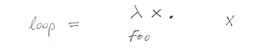
Here, both foo and x can be any expressions. I denote the argument x, and the body foo. I use a tree-like way of writing expressions, with the bodies under their bindings. Written as a single line, the above becomes

loop = (λ x. foo) x

Now let’s reduce it. I use an intermediate step in my reduction, where an expression “lights up”, because it is about to be modified by what was just applied to it.

Okay, that’s interesting. We don’t know anything about the body of the function, foo, but when reducing this simple expression, it of course just turns in to foo, by the rules of β-reduction. That’s because we just replaced the bound x with a free x.

But at least we learned something. The body, foo, must reduce to the full structure of loop, λ-abstraction and all. However, if we try to just plug that into the first λ-expression, we get

foo 
= (λ x . foo) x
= (λ x . (λ x . foo) x) x
= ...(λ x . (λ x . ( ... λ x. foo ...)) x)
= ...

and that’s the correct behavior (it’s exactly what we’re looking for), but we can’t take this approach, because it means we can’t construct the combinator as a finite expression.

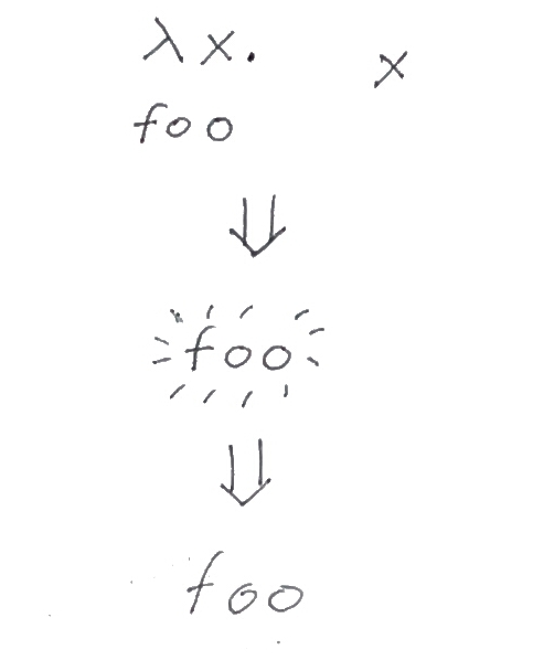
So let’s see what else we learned: foo must, at the very least, have an x to the right, because it’s supposed to look the same as what it started from, and we started with an x to the right. So let’s see what happens if we replace foo by another expression, bar x.

Great, that looks a little more as what we started with – at least now there’s still an x to the right. But we lost the λ-abstraction around bar, and we can’t just make bar a λ-abstraction with a body that contains a λ-abstraction, etc., because that would go on forever like we saw above.

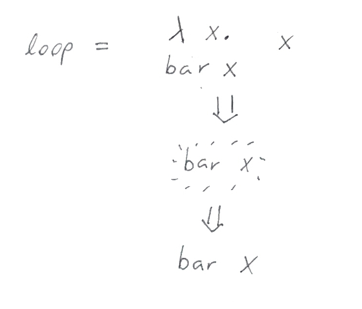
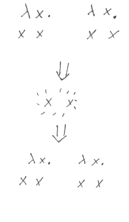
What we can try to do is to make the right x a λ-abstraction. That way, we might be able to insert it into bar. Let’s just see what happens.

Awesome! The x next to bar ensures the right side is the same after reduction, and I kept the lighting around bar to indicate it is not done reducing (because we don’t know if it contains any more instances of x that we would need to update).

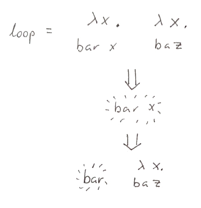
Okay, so we don’t know what bar is. Let’s try the simplest possible expression it could be, x, and see what happens.

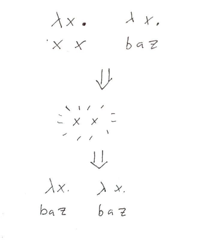
We’re getting close. Look at the expression before and after reduction: it’s strikingly similar. The only problem is that the right side completely took over and is now on both the right and left. But we are not actually using baz for anything yet, so we can just replace it with whatever. And if we want the left side to be the same as before the reduction, it looks like baz should be x x. Let’s try.

We did it! The initial expression is the same as the reduced expression, and we can now do the same reduction again, and get the same result! The final expression is

loop = (λ x . x x) (λ x . x x)

As you may have guessed, this combinator already exists, and it has a name: the ω-combinator. (ω is a small omega). The reason we started here is that it turns out, once you look at the ω-combinator, you can pretty much figure out the Y-combinator by making some small adjustments.

From ω to Y

So we just invented a lambda expression which just reproduces itself endlessly. This is almost what we want: the only adjustment we want to the result is that every new reduction should also prepend some function f to the entire expression.

Before we go on, take a moment to think about it: where could we stick an f into the expression for ω? What results do you expect?

What if we stick it in front of the body of the left expression?

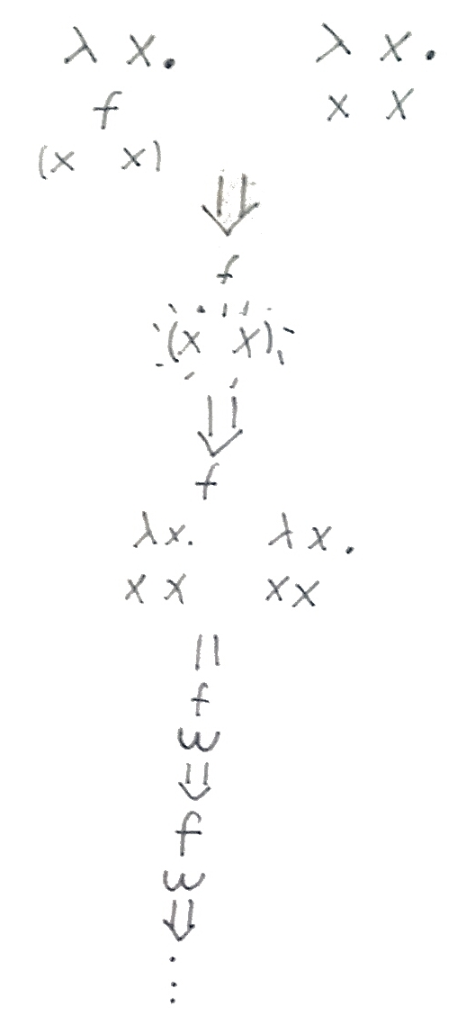
Let’s think a bit about it before we move on. If we look at the left side of the ω-combinator, it’s a function that just applies its input to itself. What we tried above just wraps that in f once, so it doesn’t work. The input, however (the right side), will keep getting applied to itself forever, so the key should be slapping the f on the body there, which should result in that f sticking around, always applying to the new input.

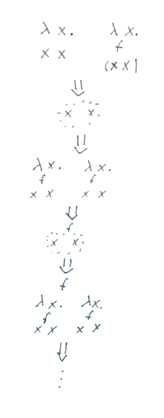
Great! Just a small issue left: we hard-coded the f in there, but we want it to be an arbitrary function that we could pass in. But that’s just the use case for variable abstraction, so we just make a λ-abstraction over f. Also, for symmetry (making a bit easier to remember), we use the result after the first reduction, which has f in both the left and right expression.

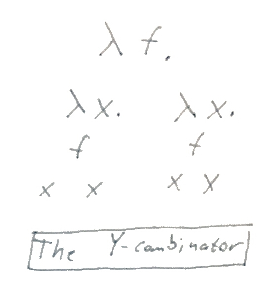
There you have it – that’s the Y-combinator in all its glory. Slap in any function and you’ll find that it reproduces endlessly.

Closing words

Thanks for following me through that little construction. It wasn’t really a proof of anything (if you want that, try proving that for any x, if x = f(x) then x = f(f(x)) = f(f(...f(x)...)), it’s straightforward). But imagine for a moment that you are Haskell Curry or Alonzo Church thinking about ways to “break” λ-calculus by making it behave weirdly, or you’re trying to answer the question of whether you can compute a factorial with λ-calculus. Fixed points might come to mind, and you would then go about constructing a fixed point combinator to show some properties of λ-calculus.

We just did the same thing, pretending these results don’t already exist, for the fun of it, and to understand it properly. I want to leave you with a quote from Richard Feynman, in the gem Feynman Lectures on Computation (1996). This is from page 15-16 in my edition:

Throughout the book, I will suggest some problems for you to play with. […] You might skip them thinking that, well, they’ve probably already been done by somebody else; so what’s the point? Well, of course they’ve been done! But so what? Do them for the fun of it. That’s how to learn the knack of doing things when you have to do them. Let me give you an example. Suppose I wanted to add up a series of numbers,

1+2+3+4+5+6+7 …

up to, say, 62. No doubt you know how to do it; but when you play with this sort of problem as a kid, and you haven’t been shown the answer … it’s fun trying to figure out how to do it. Then, as you go into adulthood, you develop a certain confidence that you can discover things; but if they’ve already been discovered, that shouldn’t bother you at all. What one fool can do, so can another, and the fact that some other fool beat you to it shouldn’t disturb you: you should get a kick out of having discovered something. Most of the problems I give you in this book have been worked over many times, and many ingenious solutions have been devised for them. But if you keep proving stuff that others have done, getting confidence, increasing the complexities of your solutions for the fun of it – then one day you’ll turn around and discover that nobody actually did that one! And that’s the way to become a computer scientist.

In that vein, I leave you with the following follow-up problem: using the Y-combinator, can you write a factorial function for natural numbers? Start by assuming you have natural numbers, the =/= (not-equal) relation and if-else constructs at your disposal. Then see if you can encode numbers in λ-calculus, then if-else, and finally the > relation. If you get stuck, you can read about Church encodings and find some strategies to help you along.

Also, make sure to look up simply typed lambda calculus, and why the Y-combinator can’t be constructed in it, and why that’s a good thing!